Table of Contents
Introduction
Measuring gas transfer rates in fermentations provides detailed information on the metabolic status of the microorganisms. In many processes the availability of oxygen is an important factor for efficient productivity. The oxygen uptake rate determines the cell specific oxygen requirement (mmol(O\(_2)\)/gDW/h) and the oxygen transfer rate describes the volume specific exchange rate (mmol(O\(_2)\)/L/h). Similarly, the CO\(_2\) exchange is measured by the biomass specific carbon emission rate (CER, (mmol(CO\(_2)\)/gDW/h)) and the volume-based carbon transfer rate (CTR, (mmol(CO\(_2)\)/L/h)). The ratio of CTR over OTR is the respiratory quotient (RQ) and provides additional information. An overview to the strategy of respiration activity monitoring system (RAMOS) is provided by Anderlei et al. (2004).
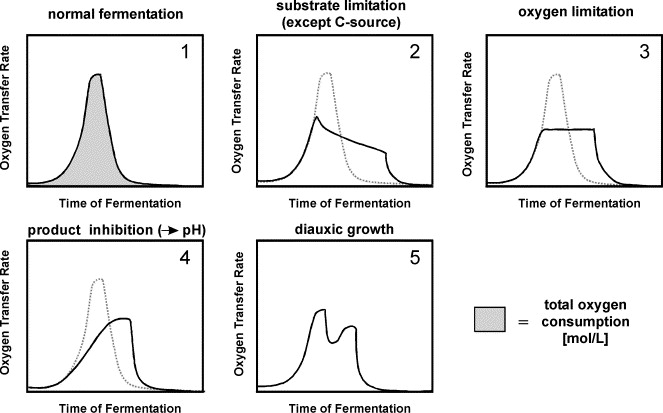
The oxygen transfer rate (OTR) can reveal different conditions of a fermentation (Anderlei & Büchs, 2001).
During fermentation, microorganisms take up the substrate(s) for growth and generate side products. Fermentation control and engineering depends on the knowledge of the different carbon routes. To test our knowledge, we can determine whether the carbon balance is closed, i.e. that the carbon processed as substrate equals all products.
To balance carbon fluxes, all metabolites with carbon need to be measured and their rates determined. This tutorial focuses on the steps when this information is available and used simulations from BiotechData.Academy to generate synthetic data. This data comes from a E. coli core genome scale model with the substrate glucose. The original model was modified by a random collection of side products.
The workflow assumes that a growth quantification, with the estimation of growth rate and substrate uptake rate, has already been performed. This tutorial show how the production rates of side products are calculated and how the biomass is included.
Download Excel: Growth dataComputational preparations
Python packages
The data analysis is based on widely available Python packages. It also requires a package called iambcodes, which can be downloaded by PyPi and provides customized nonlinear fit functions.
import os                                # navigating the operation system
import numpy as np                       # doing basic math
import pandas as pd                      # handling tables
from datetime import date                # getting the date for file saving
from scipy import stats                  # doing statistical analysis
from scipy.optimize import curve_fit     # data fitting
import matplotlib.pyplot as plt          # visualization
from iambcodes.rates import *            # improved visualization and fitting
Filesystem & parameters
The following code cell defines data file for analysis and sets the paths and figure file type of the results. Some general parameters for the conversion of mole to gramm are provided and the visualization of the “\(\pm\)” sign.
Root_Dir = os.getcwd()
Target_Dir = Root_Dir  # Adjust if needed
File = 'Example_GrowthExp.xlsx' # Add Excel file with growth data
# All files are attached with the current date
Today = date.today().strftime('%y%m%d')
# Define image properties
ImageType = 'svg'
fontsize = 15
plt.rc('font', size=fontsize)
kwargs = {'mew':5, 'lw':4}

# Substrate mol to g conversion parameter
mol2g = {'glc':1/.18, 'glyc':1/.092, 'ace':1/.059, 'eg':1/.0621}
# plus minus sign
pm = '\u00B1'
Data import
In the example file above, the sheet ‘10mM’ contains measurements for additional metabolites including CO\(_2\). The data needs to be stored in a standardized format. In this case, columns A, B, C are reserved for metadata. These inform about the experiment details and potential unit conversion requirements, e.g., to get from OD600 to cell dry weight or g/L to mM concentration. Column D represents the time column whose ID is defined in the metadata. All other columns can have data for biomass and substrate concentration with user specific column names specified in the metadata descriptions.

Standard format for data table sheet as xlsx-file type.
The following code block imports the data, stores it in a pandas dataframe and prints the available Excel Worksheets.
FileAddress = os.path.join(Target_Dir, File)
Xls_df = pd.ExcelFile(FileAddress)
print('Excel sheets:\n{}'.format(Xls_df.sheet_names))
Excel sheets:
[‘1mM’, ‘2mM’, ‘5mM’, ‘10mM’, ‘20mM’, ‘50mM’, ‘RateCompare’]
Data selection
Using the Excel Worksheet names, we select the data that we want to analyze with the variable Sheet. This is followed by a number of data corrections based on associated metadata in the standard format of the Excel sheet.
# Choosing Excel sheet
Sheet = '10mM'
# Define conversion factor, e.g. yeast: 0.62 (BNID 111182 in Bionumbers)

# Loading data from sheet into python, ignoring Metadata columns
df_orig = pd.read_excel(FileAddress, sheet_name=Sheet, usecols=lambda x: 'Metadata' not in x,)
df_orig = df_orig.dropna(how = 'all')
DelHeader = df_orig.columns[['Unnamed' in header for header in df_orig.columns]].values
df_orig = df_orig.drop(DelHeader, axis=1)

myMeta = pd.read_excel(FileAddress, sheet_name=Sheet, usecols=lambda x: 'Metadata' in x,)
TimeUnit = ''.join(myMeta.loc[myMeta['Metadata: Key']=='Time unit']['Metadata: Value'].values)
# add a biomass correction factor, e.g. from OD to gCDW, if none set to 1
BiomassUnit = ''.join(myMeta.loc[myMeta['Metadata: Key']=='Biomass unit']['Metadata: Value'].values)
if BiomassUnit == 'OD':
    ODConvert = True
    # read or define existing conversion factor for OD to gCDW/L
    BiomassCorr = myMeta.loc[myMeta['Metadata: Key']=='OD2CDW']['Metadata: Value'].values
    OD2DW = BiomassCorr if BiomassCorr.size > 0 else OD2DW
    BiomassUnit = 'gDW/L'
elif BiomassUnit == 'gDW/L':
    OD2DW = 1.
else:
    print('Use standard abbreviation for biomass unit: gDW/L, OD')
SubstrateUnit = ''.join(myMeta.loc[myMeta['Metadata: Key']=='Substrate unit']['Metadata: Value'].values)# 'mM'
# add a substrate correction factor, e.g. to convert from g/l to mM
SubstrateID = ''.join(myMeta.loc[myMeta['Metadata: Key']=='Substrate']['Metadata: Value'].values).lower()
# conversion of g/l concentration to mmol/l
SubstrateCorr = mol2g[SubstrateID] if SubstrateUnit=='g/L' else 1.
YieldCorr = 1/mol2g[SubstrateID]# if SubstrateUnit=='mM' else 1.

# Extract column ids from metadata
SubstrateColumns = myMeta['Metadata: Value'][myMeta['Metadata: Key']=='Substrate'].astype(str).values[0]
BiomassColumns = myMeta['Metadata: Value'][myMeta['Metadata: Key']=='Biomass Column ID'].astype(str).values[0]
TimeID = myMeta['Metadata: Value'][myMeta['Metadata: Key']=='Time Column ID'].astype(str).values[0]
BiomassID = [col for col in df_orig.columns if BiomassColumns in col]
SubstrateID = [col for col in df_orig.columns if SubstrateColumns in col]

df=df_orig.dropna(how = 'all').copy()

df['Biomass'] = np.mean(df[BiomassID].to_numpy(), axis=1)*OD2DW
df['Substrate'] = np.mean(df[SubstrateID].to_numpy(), axis=1)*SubstrateCorr
Gas Transfer Rates
OTR & CTR
There are different methods to measure the gas transfer rates, in the RAMOS strategy, the gas exchange is interrupted and the decline of the target gas in the gas space is measured.
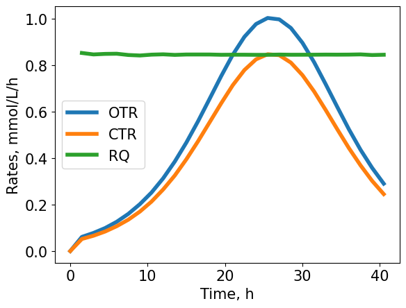
OTR, CTR and RQ for the example shakeflask cultivation. The OTR is a smooth bell-shape, thus, there is no other limitation except the carbon substrate.
Respiratory Quotient
Information of the carbon and oxygen transfer rates can provide useful insight to a bioprocess. The ratio of carbon transfer over oxygen transfer is the respiratory quotient (RQ) and is equal to 1 if glucose is fully metabolized:
$$ C_6H_{12}O_6 + 6O_2 \rightarrow 6CO_2 + 6H_2O \\ RQ = \frac{6CO_2}{6O_2} = 1 \frac{mmol(CO_2)}{mmol(O_2)} $$Different substrates will result in different RQ values when fully catabolized. If for glucose the measured RQ is 1, then the electrons end up almost entirely in CO\(_2\). If the RQ>1, then less O\(_2\) is required and reduced products are formed. If the RQ<1, then more O\(_2\) is required per CO\(_2\), which indicates that side producs are formed, that are more oxidized than glucose, high overflow metabolism, or higher maintenance requirements. The figure shows a reduced RQ for the example cultivation of about 0.85 mmol(CO\(_2\))/mmol(O\(_2\)). This indicates, that there are byproducts with a higher oxidation, presumably organic acids.
Production rates
Growth Rate and Substrate Uptake Rate
We use the example for which the growth quantification has been documented in the Tutorial Growth Quantification. The experiment starts with 10 mM of glucose substrate for growth simulation in the E. coli core genome scale model and the growth quantification uses the Verhulst equation. The Verhulst equation is more appropriate because the data follows the sigmoidal shape nicely and all data can be used for analysis. This growth rate is lower than expected, reasons may be that side products sequest substantial amount of carbon, or the substrate uptake rate is inhibited. The substrate uptake rate is also lower than expected and thus leads to lower growth rate. The yields is 0.33 gDW/gGlc, also below expected values, thus there are side products or higher CO\(_2\) production.
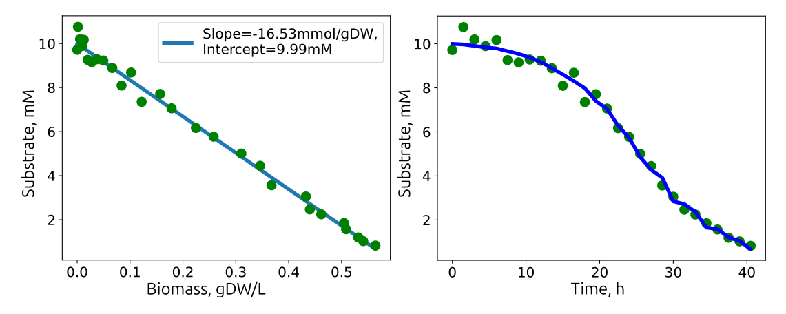
Linear relationship between biomass accumulation and substrate consumption. The slope (\(mmol/gDW\)) is multiplied with the growth rate (\(/h\)) and represents the substrate uptake rate (\(mmol/gDW/h\)).
| Growth Rate, /h | Substrate Uptake, mmol/gDW/h | Yield, gDW/gGlc | |
|---|---|---|---|
| Initial Substrate, 10 mM, Verhulst Regression | 0.17±0.00 | 2.9±0.1 | 0.33±0.01 |
# Calculating substrate uptake rate
DeltaBm = np.array(df['Biomass']-df['Biomass'][0], dtype=float)
Sub_sl, Sub_ic, Sub_r, _, Sub_sl_sterr = stats.linregress(DeltaBm, df['Substrate'])
SubUp = round(-Sub_sl*Bm_sl,1)
SubUp_sterr = round(SubUp*np.sqrt( (Sub_sl_sterr/Sub_sl)**2 + (Bm_sl_sterr/Bm_sl)**2 ), 2)

# r2 calculation
r2_Sub, _ = FitR2(df['Substrate'], DeltaBm, [Sub_sl, Sub_ic], law='lin', inlog=False)

# yield calculation
Yield = round(Bm_sl,2) / (SubUp * YieldCorr)
# calculating the standard error of the yield based on gaussian error propagation
Yield_sterr = round(Yield*np.sqrt( (SubUp_sterr/SubUp)**2 + (Bm_sl_sterr/Bm_sl)**2 ), 2)

print(f'Growth rate: {round(Bm_sl,2)}({pm}{round(Bm_sl_sterr,2)}) /{TimeUnit}, with R2: {round(r2_BM,2)}')
print(f'Substrate uptake: {SubUp}({pm}{SubUp_sterr}) mmol/gCDW/h (check units), with R2: {round(abs(Sub_r),2)}')
print(f'Biomass yield: {round(Yield,2)}{pm}{Yield_sterr} gDW/g')

# Substrate plots
LinReg = lambda x, m, b: m*x + b
plt.plot(DeltaBm, LinReg(DeltaBm, Sub_sl, Sub_ic), **kwargs)
plt.plot(DeltaBm, df['Substrate'],'go', **kwargs)
plt.legend([f'Slope={Sub_sl:.2f}mmol/gDW,\nIntercept={Sub_ic:.2f}mM'])
plt.xlabel('$\\Delta$ Biomass, gDW/L')
plt.ylabel('Substrate, mM')
plt.show()

plt.plot(df['time'], df['Substrate'], 'og', label='Substrate', **kwargs)
plt.plot(df['time'], Sub_ic+Sub_sl*DeltaBm, '-b', label=f'fit, rate={SubUp}{pm}{SubUp_sterr}mmol/gCDW/h', **kwargs)
plt.xlabel(f'Time, {TimeUnit}')
plt.ylabel('Substrate, mM')
plt.show()
Side Product Quantification
For the example growth quantification, the following additional side products are generated: \(\alpha\)-ketoglutarate (AKG), CO\(_2\), formate (For), pyruvate (Pyr) and succinate (Suc) with duplicate concentration measurements.
The production rates for side products are calculated as the linear regression between the biomass accumulation and the product accumulation:
\[ C_{Met} = N(t) Y_{Met/Bm}\]with \( N(t)\) as the biomass and \(Y_{Met/Bm}\) the metabolite-biomass yield in mmol/gDW. Products that are produced at a constant rate will display a linear relationship in a plot of the product versus the Biomass with slope \(Y_{Met/Bm}\). The production rates are \(R_{Met} = Y_{Met/Bm} \cdot \mu\), the product of yield and the growth rate. Of interest is also the conversion of the absolute biomass associated rate into a C-molar rate by multiplication with the carbon content:
$$ q_{Metabolite}\left[\frac{Cmmol}{gDW h}\right] = R_{Metabolite}\left[\frac{mmol}{gDW\cdot h}\right] C_{Metabolite} \left[\frac{Cmmol}{mmol}\right] $$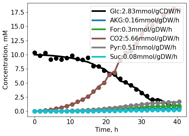
The product concentrations are estimated based on the individual metabolite-biomass yields from the linear relationship.
The rates of carbon flow to substrate, products and biomass needs to be balanced. To check this, the carbon associated rates are multiplied by the carbon content to get the carbon-molar rates (Cmmol/gDW/h). For Biomass the number of carbon for growth is calculated from the genome scale model biomass equation by summing up all carbon (42.6 C-mmol/gDW) and multiplication by the growth rate. The table below shows the respective values of carbon rates and is 1.3 Cmmol/gDW/h (~8%) of substrate is not balanced. This error is caused by random measurement noise and rounding.
If the gas transmissions are in equilibrium, it is possible to correlate the CTR with the biomass specific carbon emission rate (CER) and the OUR with the biomass specific oxygen uptake rate (OUR). With the RQ (0.85 mmol(CO\(_2\))/mmol(O\(_2\))) and the absolute CER (5.7 mmol(CO\(_2\))/gDW/h):
$$ OUR = \frac{CER}{RQ} = \frac{ 5.7 \left[\frac{mmol(CO_2)}{gDW\cdot h}\right]}{0.85 \left[\frac{mmol(CO_2)}{mmol(O_2)}\right]} = 6.7 \left[\frac{mmol(O_2)}{gDW\cdot h}\right] $$The simulations use the E. coli core genome scale model Orth et al., 2010 with the following biomass composition. Summing the carbon content of the biomass components provides the biomass carbon content (42.6 Cmmol/gDW).
| Biomass Component | 3PG | AcCoA | E4P | F6P | G3P | G6P | Gln | Glu | OAA | PEP | PYR | R5P | Biomass |
|---|---|---|---|---|---|---|---|---|---|---|---|---|---|
| Stoichiometry | 1.496 | 3.7478 | 0.361 | 0.0709 | 0.129 | 0.205 | 0.2557 | 0.8232 | 1.7867 | 0.5191 | 2.8328 | 0.8977 | 1 |
| Carbon content | 3 | 2 | 4 | 6 | 3 | 6 | 5 | 5 | 4 | 3 | 3 | 5 | 42.6 |
prod = myMeta.loc[myMeta['Metadata: Key']=='Product', 'Metadata: Value'].squeeze()
Products = [p.strip() for p in prod.split(',')] if isinstance(prod, str) and prod.strip().lower() not in ('', 'nan') else []
if Products:
    Prod_df = pd.DataFrame()
    Prod_dict = {p: {} for p in Products}   # initialize keys

    for myProd in Products:
        myCols = [col for col in df_orig.columns if myProd in col]
        if len(myCols) == 0:
            print(f'Warning: no columns found for product {myProd}')
            continue

        myDat = df[myCols].to_numpy()
        Prod_df[f'{myProd}_mean'] = np.mean(myDat, axis=1)

        # linear fit of product vs DeltaBm
        Prod_sl, Prod_ic, Prod_r, _, Prod_sl_sterr = stats.linregress(DeltaBm, Prod_df[f'{myProd}_mean'])

        # compute rate and stderr safely
        rate = round(Prod_sl*Bm_sl, 1)
        if Prod_sl == 0 or Bm_sl == 0:
            rate_sterr = np.nan
        else:
            rate_sterr = round(rate * np.sqrt((Prod_sl_sterr / Prod_sl) ** 2 + (Bm_sl_sterr / Bm_sl) ** 2), 2)

        Prod_dict[myProd]['rate'] = rate
        Prod_dict[myProd]['rate_sterr'] = rate_sterr
        Prod_dict[myProd]['r2'] = round(abs(Prod_r), 2)

        print(f"Product {myProd} formation rate: {Prod_dict[myProd]['rate']}({pm}{Prod_dict[myProd]['rate_sterr']}) mmol/gCDW/h, R2: {Prod_dict[myProd]['r2']}")

    # create a consistent color for each product using a colormap
    cmap = plt.get_cmap('tab10', len(Products))
    colors = {p: cmap(i) for i, p in enumerate(Products)}

    for myProd in Products:
        col = colors[myProd]
        plt.plot(DeltaBm, Prod_df[f'{myProd}_mean'], 'o', color=col, label='_nolegend_', **kwargs)
        plt.plot(DeltaBm, Prod_dict[myProd]['rate']/Bm_sl * DeltaBm, '-', color=col, **kwargs)
    plt.xlabel('$\\Delta$ Biomass, gDW/L')
    plt.ylabel('Product concentration, mM')
    plt.legend(Products, loc='best')
    plt.show()

    plt.plot(df['time'], df['Substrate'], 'ok', label='_nolegend_', **kwargs)
    plt.plot(df['time'], Sub_ic+Sub_sl*DeltaBm, '-k', label=f'Glc:{SubUp}mmol/gCDW/h', **kwargs)
    for myProd in Products:
        col = colors[myProd]
        plt.plot(df['time'], Prod_df[f'{myProd}_mean'], 'o', color=col, label='_nolegend_', **kwargs)
        plt.plot(df['time'], Prod_dict[myProd]['rate']/Bm_sl * DeltaBm, '-', color=col, label=f'{myProd}:{Prod_dict[myProd]["rate"]}mmol/gDW/h', **kwargs)
    plt.xlabel('Time, h')
    plt.ylabel('Concentration, mM')
    plt.legend(loc='best')

    plt.tight_layout()
    plt.show()
Electron Balance & Degree of Reduction
Microbial fermentations must be balanced on the carbon and the electron fluxes. The electron distribution can be followed using the degree of reduction of the metabolites which designates the number of free electrons in a component normalized to 1 C-mol. The degree of reduction for a component is calculated by:
$$ C_aH_bO_cN_d\\[.3cm] \gamma = \frac{4a + b - 2c - 3d}{a} $$The electron balance is based on the equality of electrons from substrate and oxygen to biomass and products. This is calculated based on the degree of reduction (\(\gamma\)) multiplied with the C-molar based flux q (Cmmol/gDW/h):
$$ \gamma_{S}q_{S} + \gamma_{O_2}R_{O_2} = \gamma_{X}q_{X} + \sum_{i}\gamma_{P_i}q_{P_i} $$With degrees of reduction (\(\gamma\)), C-molar rates (q), or standard rate (R) for substrate (S), oxygen (O\(_2\)), Biomass (X), and Products (P\(_i\)). The degree of reduction for the biomass of the E. coli core model was determined based on the biomass equation. By rearranging the balance equation of the degrees of reduction, it is possible to determine the oxygen uptake rate (\(R_{O_2}\)):
$$ R_{O_2} = \frac{\gamma_{X}q_{X} + \sum_{i}\gamma_{P_i}q_{P_i} - \gamma_{S}q_{S}}{\gamma_{O_2}} $$Based on this equation, the requirement for the oxygen rate for full electron balance is 7.19 mmol/gDW/h, over 25% higher than the actual OUR.
| Metabolite | Formula | Rate, mmol/gDW/h (actual) | q, C-Rate, Cmmol/gDW/h | \(\gamma\) (\(e^-\)/Cmmol) | \(\gamma \cdot q\) (\(e^-\)/gDW/h) |
|---|---|---|---|---|---|
| Oxygen | O\(_2\) | 6.7±0.2 (6.2) | -4 | -26.8 | |
| CO\(_2\) | CO\(_2\) | 5.7±0.2 (5.8) | 5.7 | 0 | 0 |
| Glucose | C\(_6\)H\(_{12}\)O\(_6\) | 2.8±0.1 (2.6) | 16.8 | 4 | 67.2 |
| AKG | C\(_5\)H\(_6\)O\(_5\) | 0.16±0.01 (0.16) | 0.8 | 3.2 | 2.6 |
| For | CH\(_2\)O\(_2\) | 0.3±0.01 (0.3) | 0.3 | 2 | 0.6 |
| Pyr | C\(_3\)H\(_4\)O\(_3\) | 0.51±0.02 (0.47) | 1.5 | 3.33 | 5 |
| Suc | C\(_4\)H\(_6\)O\(_4\) | 0.08±0.00 (0.08) | 0.02 | 3.5 | 0.07 |
| Biomass | CH\(_{1.77}\)O\(_{0.49}\)N\(_{0.24}\) | 0.17±0.01 (0.16) | 7.2 | 4.07 | 29.3 |
| Sum | 1.3 (7.6% error) | 2.8 (7% error) |
Summary
Overall, the actual rates from the original simulation could be well estimated. The constant RQ shows that the metabolism is constant throughout the simulation and its lower value indicates the existence of organic acid byproducts. The carbon and electron balances calculation result in 7% imbalances that occur in data even when experimental noise is deactivated. The reason is that the growth rate is slightly overestimated, probably because the biomass estimation on the basis of the logistic growth equation with a maximum biomass capacity in the model does not optimally capture the decrease of growth rate due to substrate depletion.