Table of Contents
Introduction
Microorganisms growth by converting carbon substrates to biomass and side products. The conversion process during metabolism is unique for each organism and in each condition and leads to a range of growth rates and yields of biomass from substrate. For biotechnological purposes it is important to know the growth rates, biomass yields and side products in order to effectively plan fermentations.
Although the measurement of biomass, substrate and sideproducts are basic microbiological experiments, the growth quantification requires a few hurdles and advanced analysis steps. It is important to adhere to units consistently, because there are many conversion steps and external parameters. The rates themselves are estimated using regression of suitable microbial growth laws.
A practical implementation is reported in Liebal et al. (2022) for the genome scale metabolic model reconstruction of Ustilago maydis. Experiments were performed to quantify the growth for model validation, with concentrations from 10-50 mM. Figure 3 in the article (below) shows the association of glucose uptake to growth rate and effect of initial glucose concentration on glucose uptake rate.
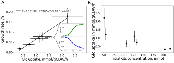
Microbial growth characterization for U. maydis in Liebal et al. (2022, Figure 3). Seven different growth experiments on glucose (10-50 mM) with estimations of growth rate, substrate uptake rate and yield.
This tutorial guides the data analysis for microbial growth quantification. The data is generated by the BiotechData.Academy virtual cell simulation on a E. coli core genome scale model with the substrate glucose. The original model was modified by a random collection of side products, so that the maximum theoretical yield is not reached.
The workflow starts by calculating the growth rate, substrate uptake rate and yield for each growth experiment. The results of the different experiments are integrated by
- investigating the relationship between the substrate uptake rate and the growth rate,
- identifying the substrate uptake kinetics by analyzing the relationship among initial substrate concentration and substrate uptake rate.
Computational preparations
Python packages
The data analysis is based on widely available Python packages. It also requires a package called iambcodes, which can be downloaded by PyPi and provides customized nonlinear fit functions.
import os                                # navigating the operation system
import numpy as np                       # doing basic math
import pandas as pd                      # handling tables
from datetime import date                # getting the date for file saving
from scipy import stats                  # doing statistical analysis
from scipy.optimize import curve_fit     # data fitting
import matplotlib.pyplot as plt          # visualization
from iambcodes.rates import *            # improved visualization and fitting
Filesystem & parameters
The following code cell defines data file for analysis and sets the paths and figure file type of the results. Some general parameters for the conversion of mole to gramm are provided and the visualization of the “\(\pm\)” sign.
Root_Dir = os.getcwd()
Target_Dir = Root_Dir  # Adjust if needed
File = 'Example_GrowthExp.xlsx' # Add Excel file with growth data
# All files are attached with the current date
Today = date.today().strftime('%y%m%d')
# Define image properties
ImageType = 'svg'
fontsize = 15
plt.rc('font', size=fontsize)
kwargs = {'mew':5, 'lw':4}

# Substrate mol to g conversion parameter
mol2g = {'glc':1/.18, 'glyc':1/.092, 'ace':1/.059, 'eg':1/.0621}
# plus minus sign
pm = '\u00B1'
Data import
The data needs to be stored in a standardized format. In this case, columns A, B, C are reserved for metadata. These inform about the experiment details and potential unit conversion requirements, e.g., to get from OD600 to cell dry weight or g/L to mM concentration. Column D represents the time column with the required name time. All other columns can have data for biomass and substrate concentration with user specific column names.
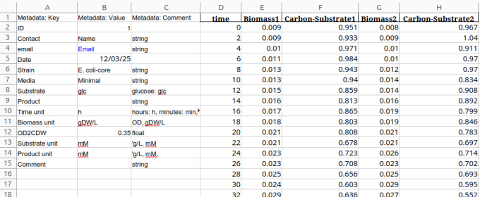
Standard format for data table sheet as xlsx-file type.
The following code block imports the data, stores it in a pandas dataframe and prints the available Excel Worksheets.
FileAddress = os.path.join(Target_Dir, File)
Xls_df = pd.ExcelFile(FileAddress)
print('Excel sheets:\n{}'.format(Xls_df.sheet_names))
Excel sheets:
[‘1mM’, ‘2mM’, ‘5mM’, ‘10mM’, ‘20mM’, ‘50mM’, ‘RateCompare’]
Data selection
Using the Excel Worksheet names, we select the data that we want to analyze with the variable Sheet. This is followed by a number of data corrections based on associated metadata in the standard format of the Excel sheet.
# Choosing Excel sheet
Sheet = '10mM'
# Define conversion factor, e.g. yeast: 0.62 (BNID 111182 in Bionumbers)

# Loading data from sheet into python, ignoring Metadata columns
df_orig = pd.read_excel(FileAddress, sheet_name=Sheet, usecols=lambda x: 'Metadata' not in x,)
df_orig = df_orig.dropna(how = 'all')
DelHeader = df_orig.columns[['Unnamed' in header for header in df_orig.columns]].values
df_orig = df_orig.drop(DelHeader, axis=1)

myMeta = pd.read_excel(FileAddress, sheet_name=Sheet, usecols=lambda x: 'Metadata' in x,)
TimeUnit = ''.join(myMeta.loc[myMeta['Metadata: Key']=='Time unit']['Metadata: Value'].values)
# add a biomass correction factor, e.g. from OD to gCDW, if none set to 1
BiomassUnit = ''.join(myMeta.loc[myMeta['Metadata: Key']=='Biomass unit']['Metadata: Value'].values)
if BiomassUnit == 'OD':
    ODConvert = True
    # read or define existing conversion factor for OD to gCDW/L
    BiomassCorr = myMeta.loc[myMeta['Metadata: Key']=='OD2CDW']['Metadata: Value'].values
    OD2DW = BiomassCorr if BiomassCorr.size > 0 else OD2DW
    BiomassUnit = 'gDW/L'
elif BiomassUnit == 'gDW/L':
    OD2DW = 1.
else:
    print('Use standard abbreviation for biomass unit: gDW/L, OD')
SubstrateUnit = ''.join(myMeta.loc[myMeta['Metadata: Key']=='Substrate unit']['Metadata: Value'].values)# 'mM'
# add a substrate correction factor, e.g. to convert from g/l to mM
SubstrateID = ''.join(myMeta.loc[myMeta['Metadata: Key']=='Substrate']['Metadata: Value'].values).lower()
# conversion of g/l concentration to mmol/l
SubstrateCorr = mol2g[SubstrateID] if SubstrateUnit=='g/L' else 1.
YieldCorr = 1/mol2g[SubstrateID]# if SubstrateUnit=='mM' else 1.

# Extract column ids from metadata
SubstrateColumns = myMeta['Metadata: Value'][myMeta['Metadata: Key']=='Substrate'].astype(str).values[0]
BiomassColumns = myMeta['Metadata: Value'][myMeta['Metadata: Key']=='Biomass Column ID'].astype(str).values[0]
TimeID = myMeta['Metadata: Value'][myMeta['Metadata: Key']=='Time Column ID'].astype(str).values[0]
BiomassID = [col for col in df_orig.columns if BiomassColumns in col]
SubstrateID = [col for col in df_orig.columns if SubstrateColumns in col]

df=df_orig.dropna(how = 'all').copy()

df['Biomass'] = np.mean(df[BiomassID].to_numpy(), axis=1)*OD2DW
df['Substrate'] = np.mean(df[SubstrateID].to_numpy(), axis=1)*SubstrateCorr
Growth Laws and Substrate Uptake
Microbial growth follows three stages: lag-, log- and stationary phase. The lag-phase is a time period directly after culture incubation after for example a overnight culture. The cells adapt to the new conditions and growth is shortly slower than expected. After the cells have adapted, they growth exponentially leading to the log-phase during which the biomass doubles in fixed intervalls. The exponential growth can only continue when the substrate concentration is high, there is space enough to growth, and toxic side products or growth inhibitors have not accumulated. At some point, the growth conditions deteriorate, any of the mentioned conditions fails, e.g., the substrate nears exhaustion, the growth rate decreases and the culture enters the stationary phase. During the stationary phase the biomass stays constant. This my be followed by a death phase, during which cells die and the biomass signal decreases.
Exponential Growth Law
To quantify the growth rate different laws can be used. Among the most basic laws is the exponential growth law:
\[N(t) = N_0 e^{\mu t}\]Here, \( N(t)\) is the biomass at time \(t\), \(N_0\) is the initial biomass and \(\mu\) is the growth rate. The exponential growth rate can be fitted to the data during unlimited growth conditions of the log phase. A simple procedure is to take the natural logarithm of both sides:
\[ln(N(t)) = ln(N_0) + \mu t\]A plot should display an approximately linear relationship of the biomass (\(ln(N(t))\)) over time. If deviations from linearity occurs, the data needs to be restricted to the linear range. Hence not all data is used for the regression.
Logistic Growth/Verhulst Equation
If the data contains a stationary phase, it is more suitable to estimate growth parameters with a logistic growth model (Verhulst equation).
\[N(t) = \frac{C}{1+ \left( \frac{K-N_0}{N_0}\right) e^{-\mu t}}\]With the Verhulst equation all data can be fitted to the logistic growth model and the resulting parameters are more statistically stable. This requires a non-linear least squares fit of the data.
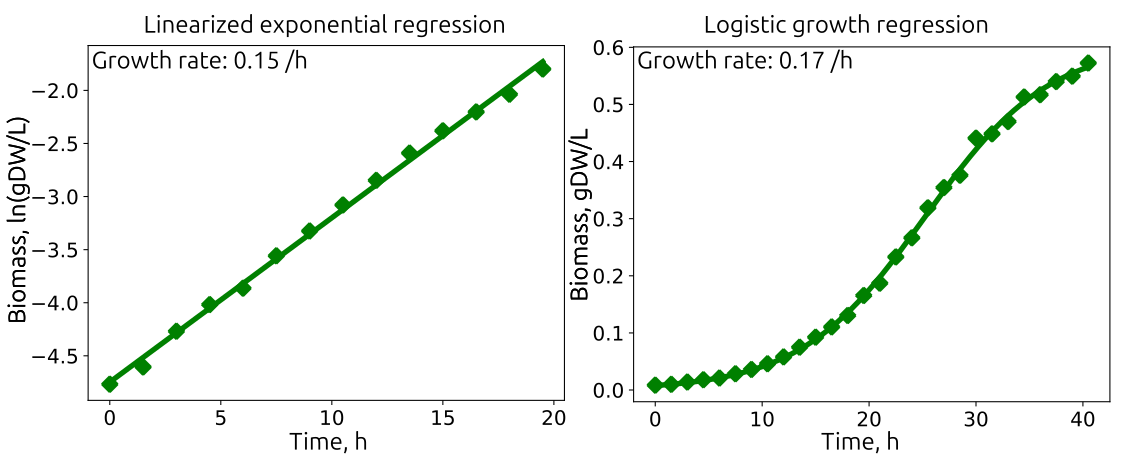
Examples to estimate growth rate and substrate uptake for a growth experiment. The data is identical in both cases. For Linearized exponential regression only data can be included with a linear ln(biomass) to time relation, hence the data considered for regression only included 0–20 h. The Logistic growth regression can include the stationary phase, in this case the whole data set and is therefore statistically stronger.
# Choose Growth Law
# Linearized Exponential: 'lex'
# Verhulst Logistic: 'log'
# Exponential: 'exp'
# Linear: 'lin'
BMLaw ='log'
# Enter the start and end times for exponential growth [1.5,8.6]:
ExpGrwth = [0,50]

inlog = False
if BMLaw == 'lex':
    inlog = True
    BMLaw = 'lin'
p0 = None # enter initial guesses for the logarithmic parameters here

# Extracting data for analysis
ExpGrwth_ind = SubVector(ExpGrwth,df['time'].values)
Time = np.array(df['time'][ExpGrwth_ind]) # - df['time'][ExpGrwth_ind[0]]
Biomass = np.array(df['Biomass'][ExpGrwth_ind], dtype=float)
Substrate = np.array(df['Substrate'][ExpGrwth_ind])

# Calculating growth rate
Bm_sl, Bm_sl_sterr, Bm_ic, Bm_lim = FitGrowth(Time, Biomass, law=BMLaw, inlog=inlog, p0=p0)
PlotPar = [Bm_sl, Bm_ic, Bm_lim] if BMLaw=='log' else [Bm_sl, Bm_ic]
r2_BM, _ = FitR2(Time, Biomass, PlotPar, law=BMLaw, inlog=inlog)

# Biomass plot
FigureGrowth = '{}_{}_{}_GrowthFit.{}'.format(Today, Sheet, BMLaw, ImageType)
FigureGrowthPath = os.path.join(Target_Dir, FigureGrowth)
PlotFit(Time, Biomass, PlotPar, Bm_sl_sterr, [TimeUnit, BiomassUnit], law=BMLaw, inlog=inlog, export_file=FigureGrowthPath, kwargs=kwargs)
plt.ylabel('ln(mM)')
plt.show()
Calculating Substrate Uptake Rate and Yield
The substrate uptake rates are calculated as the linear regression between the biomass accumulation and the substrate decrease from begin of the experiment:
\[ Substrate = N(t) Y_{Sub/Bm} + C_{Sub}(0)\]with \(N(t)\) as the biomass, \( Y_{Sub/Bm} \) the substrate-biomass yield in mmol/gDW and \(C_{Sub}(0)\) the initial substrate concentration. The substrate uptake rate is \(R_{Sub} = Y_{Sub/Bm} \cdot \mu\), the product of the substrate-biomass yield and the growth rate.
The biomass-substrate yield is calculated by dividing the growth rate (\(/h\)) with the substrate uptake rate (\(mmol/gDW/h\)). The molar yield (\(gDW/mmol\)) is multiplied with the substrate molar mass (\(g/mol\)) to get the more common mass yield (\(gGlc/gDW\)).
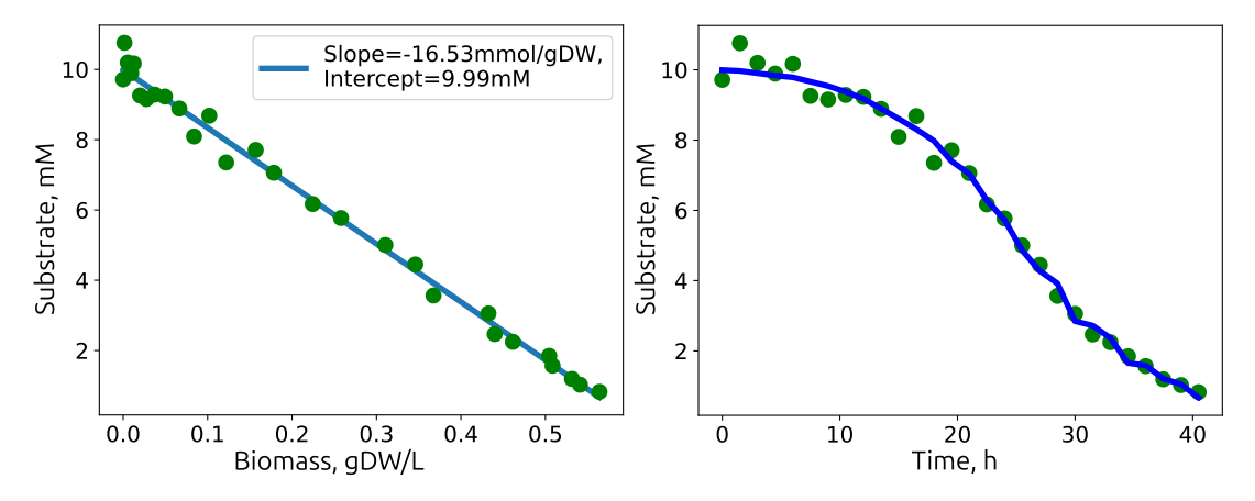
Linear relationship between biomass accumulation and substrate consumption. The slope (\(mmol/gDW\)) is multiplied with the growth rate (\(/h\)) and represents the substrate uptake rate (\(mmol/gDW/h\)) .
# Calculating substrate uptake rate
DeltaBm = np.array(df['Biomass']-df['Biomass'][0], dtype=float)
Sub_sl, Sub_ic, Sub_r, _, Sub_sl_sterr = stats.linregress(DeltaBm, df['Substrate'])
SubUp = round(-Sub_sl*Bm_sl,2)
SubUp_sterr = round(SubUp*np.sqrt( (Sub_sl_sterr/Sub_sl)**2 + (Bm_sl_sterr/Bm_sl)**2 ), 2)

# r2 calculation
r2_Sub, _ = FitR2(df['Substrate'], DeltaBm, [Sub_sl, Sub_ic], law='lin', inlog=False)

# yield calculation
Yield = round(Bm_sl,2) / (SubUp * YieldCorr)
# calculating the standard error of the yield based on gaussian error propagation
Yield_sterr = round(Yield*np.sqrt( (SubUp_sterr/SubUp)**2 + (Bm_sl_sterr/Bm_sl)**2 ), 2)

print(f'Growth rate: {round(Bm_sl,2)}({pm}{round(Bm_sl_sterr,2)}) /{TimeUnit}, with R2: {round(r2_BM,2)}')
print(f'Substrate uptake: {SubUp}({pm}{SubUp_sterr}) mmol/gCDW/h (check units), with R2: {round(abs(Sub_r),2)}')
print(f'Biomass yield: {round(Yield,2)}{pm}{Yield_sterr} gDW/g')

# Substrate plots
LinReg = lambda x, m, b: m*x + b
plt.plot(DeltaBm, LinReg(DeltaBm, Sub_sl, Sub_ic), **kwargs)
plt.plot(DeltaBm, df['Substrate'],'go', **kwargs)
plt.legend([f'Slope={Sub_sl:.2f}mmol/gDW,\nIntercept={Sub_ic:.2f}mM'])
plt.xlabel('$\Delta$ Biomass, gDW/L')
plt.ylabel('Substrate, mM')
plt.show()

plt.plot(df['time'], df['Substrate'], 'og', label='Substrate', **kwargs)
plt.plot(df['time'], Sub_ic+Sub_sl*DeltaBm, '-b', label=f'fit, rate={SubUp}{pm}{SubUp_sterr}mmol/gCDW/h', **kwargs)
plt.xlabel(f'Time, {TimeUnit}')
plt.ylabel('Substrate, mM')
plt.show()
Growth Quantification for Single Experiment
The quantification of the experiment introduded before, with 10 mM of glucose substrate for growth simulation in the E. coli core genome scale model results in growth rates of 0.15 /h for regression with exponential equation and 0.17 /h with Verhulst equation.. The Verhulst equation is more appropriate because the data follows the sigmoidal shape nicely and all data can be used for analysis. This growth rate is much lower than what could be expected by E. coli, reasons may be that side products sequest substantial amount of carbon, or the substrate uptake rate is inhibited. The substrate uptake rate is at ~2.9 mmol/gDW/h is also lower than expected and thus leads to lower growth rate. The yields is 0.33 gDW/gGlc, also below expected values, thus there are side products or higher CO\(_2\) production.
| Regression type | Exponential Law | Verhulst Equation |
|---|---|---|
| Initial Substrate, mM | 10 | |
| Experiment duration, h | 40 | |
| Growth rate analysis time, h | 0-20 | 0-40 |
| Growth rate, /h | 0.15±0.00 | 0.17±0.00 |
| Substrate uptake, mmol/gDW/h | 2.56±0.06 | 2.85±0.08 |
| Yield, gDW/gGlc | 0.33±0.01 | 0.33±0.01 |
Experiment Integration for Substrate Kinetics
Additional information about growth properties and substrate kinetics can be determined when growth experiments at different substrate concentrations with different growth rates are combined. Using the virtual lab simulations of BiotechData.Academy the previously described growth quantification was repeated for different substrate concentrations. The results of initial substrate concentration, growth rate, substrate uptake rate and yield, along with their standard variations were stored in a separate table sheet with a standardized format. The python code shows the commands used to load the standard format into python.
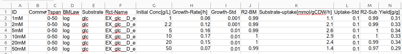
Standard format to integrate different growth quantification analyses for data table sheet as xlsx-file type.
Sheet = 'RateCompare' # Choose Excel sheet
RateComp = pd.read_excel(FileAddress, sheet_name=Sheet)
print('Data columns in Excel sheet:\n{}'.format(RateComp.columns))
print('Available growth experiments:\n{}'.format(RateComp['ID'].values))
# Output Files
# All files are attached with the current date
Today = date.today().strftime('%y%m%d')
# Figure files
FigureAccel = '{}_{}_GrowthVsSubRate.{}'.format(Today, os.path.splitext(os.path.split(File)[1])[0], ImageType)
FigureAccelPath = os.path.join(Target_Dir, FigureAccel)

InhibitCorrFig = '{}_{}_SubRateVSInitSub.{}'.format(Today, os.path.splitext(os.path.split(File)[1])[0], ImageType)
InhibitCorrPath = os.path.join(Target_Dir, InhibitCorrFig)
Yield and NGAM
When combining growth data of different experiments the yield can be independently calculated and the non-growth associated maintenance requirements of the substrate. All growth rates are plotted versus the substrate uptake rates and a linear relationship should be evident and the slope is equal to the yields of the single experiments. If no linear relationship can be observed, then the yield has changed within the experiments indicating a different metabolic state. In the figure below, the yield of the linear regression is 0.37 gDW/gGlc, slightly higher than the individually calculated yields, although the data is simulated. The calculated yield is lower than experimental values of 0.45 g/g (B10numb3r5), and indicates the production of side products or larger CO\(_2\) production.
The interception of the linear regression with the substrate uptake rate indicates the substrate requirement in the absence of growth and is related to the non-growth associated maintenance (NGAM). In this example, the value is 0.25 mmolGlc/gDW/h. Aerobic respiration yields around 30-32 ATP/Glc Wikipedia in E. coli, which means that ~8 mmolATP/gDW/h is the ATP related NGAM. Indeed, the NGAM (in reaction ATPM) used in the genome scale model for simulation uses a value of 8.4 mmolATP/gDW/h Orth et al., 2010.

Linear relationship between growth rate and substrate consumption. The slope (\(gDW/mmol\)) corresponds with the yields of the single experiments if the metabolic condition is comparable. Extending the linear regression to zero growth rate reveals the non-growth associated maintenance cost (NGAM).
# Define names of columns for analysis
GrowthMean = 'Growth-Rate[/h]'
GrowthStdv = 'Growth-Std'
SubstrMean = 'Substrate-uptake[mmol/gCDW/h]'
SubstrStdv = 'Uptake-Std'
SubstrInit = 'Initial Conc[g/L]'

RateComp_corr = RateComp

GrowthVal = RateComp_corr[GrowthMean].values
SubVal = RateComp_corr[SubstrMean].values
GVstd =  RateComp_corr[GrowthStdv].values
SVstd = RateComp_corr[SubstrStdv].values

Yield, S0, r2, _, Yield_sterr = stats.linregress(SubVal, GrowthVal)
Yield_gg = round(Yield/.18,2)
Yield_sterr_gg = round(Yield_sterr/.18,2)
# calculation of NGAM via the substrate uptake at zero growth,
# Growth = Yield*SubUp + Int -> Growth=0, then SubUp(Growth=0) = -Int / Yield
NGAM = round(-S0/Yield,2)
NGAM_std = round((-S0/(Yield-Yield_sterr) - -S0/(Yield+Yield_sterr))/2,2)
print('Yield: {} gCDW/g (+/-{}) and R2: {}'.format(Yield_gg, Yield_sterr_gg, round(r2,2)))
print('NGAM glucose requirement: {} mmol/gCDW/h+/-{}'.format(NGAM, NGAM_std))
# Growth rate VS Substrate uptake plot
plt.errorbar(SubVal, GrowthVal, xerr=SVstd, yerr=GVstd, fmt='ok') #, 'xk', label='Substrate uptake'
plt.plot(SubVal, S0+Yield*SubVal, '-k', label='fit, Y = {}(+/-{})gCDW/g'.format(Yield_gg, Yield_sterr_gg))
plt.title('Growth rate VS substrate uptake')
plt.xlabel('Substrate uptake, mmol/gCDW/h')
plt.ylabel('Growth rate, /h')
plt.legend()
plt.show()
Enzyme Kinetics
When plotting the Substrate uptake rate versus the initial substrate concentration, details on the enzyme kinetics can be determined. The figure below shows that initially, rising substrate levels lead to increasing substrate uptake rates. However, at around 10 mM, the uptake rate decreases due to non-competitive substrate inhibition. The maximum substrate uptake rate (~7 mmol/gDW/h) cannot be reached because the Michaelis-Menten constant (Ks) is to close to the substrate binding inhibition constant (Ki). This inhibition causes the low substrate uptake and consequently the lower than expected growth rates.

Enzyme kinetic effect of substrate concentration on substrate uptake rate. The maximum uptake rate decreases with increasing substrate concentration and signifies non-competitive substrate inhibition.
###############################
# Plot of initial substrate concentration versus substrate uptake rate
###############################
InitSub = RateComp_corr[SubstrInit].values
GrVal = RateComp_corr[GrowthMean].values
Grstd = RateComp_corr[GrowthStdv].values
SubVal = RateComp_corr[SubstrMean].values
SVstd = RateComp_corr[SubstrStdv].values

# define michaelis menten equation with lambda
MiMe = lambda x, Vmax, Ks: Vmax * x / (Ks + x)
NCOMP = lambda x, Vmax, Ks, Ki: Vmax * x / (Ks + x) / (1 + x/Ki)
# curve fitting
popt, pcov = curve_fit(NCOMP, InitSub, SubVal, sigma=SVstd, absolute_sigma=True)
perr = np.sqrt(np.diag(pcov))

# Estimate the parameters of the hyperbolic curve
Vmax = popt[0]
# standard deviation of the Vmax
Vmax_std = perr[0]
# Michaelis-Menten constant
Ks = popt[1]
# standard deviation of the Km
Ks_std = perr[1]
# Inhibition constant
Ki = popt[2]
# standard deviation of the Ki
Ki_std = perr[2]

# generating sample concentration values for the plot
x = np.linspace(0, np.max(InitSub), 50)
# Plot the transformed data and the fitted curve
plt.plot(x, NCOMP(x, Vmax, Ks, Ki), ':r', label=f'maxSub = {Vmax:.1f}±{Vmax_std:.1f} mmol/gDW/h,\n Ks = {Ks:.1f}±{Ks_std:.1f} mM,\n Ki = {Ki:.1f}±{Ki_std:.1f} mM')


# Initial substrate concentration VS substrate uptake plot
plt.errorbar(InitSub, SubVal, yerr=SVstd, fmt='ok')
plt.xlabel('Initial substrate concentration, mM')
plt.ylabel('Substrate uptake, mmol/gCDW/h')
plt.legend()
plt.savefig(InhibitCorrPath)
plt.show()
print('Growth rate versus substrate uptake figure saved as {}'.format(InhibitCorrPath))
Summary
Overall, the parameters could be reproduced reasonably well. The yield is lower because there are unknown side products generated. Variations in the other parameters are generated because the simulated data is added with noise, a Gauss normal-distribution with the mean of the respective measurement and variance 0.1.
| Parameter | Estimated Value | Reference |
|---|---|---|
| Yield, gDW/gGlc | 0.37 | 0.45 (B10numb3r5) |
| Vmax Glc uptake rate, mmol/gDW/h | 7±2 | 5 (preset) |
| Ks Glc uptake, mM | 4.8±2 | 2.5 (preset) |
| Ki Glc inhibition, mM | 14±6 | 23 (preset) |